Emily McRae's GIS Blog

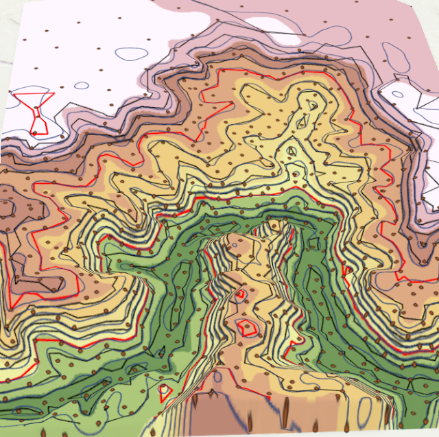
Triangular irregular networks (TIN) and digital elevation models (DEM) are explored and compared as models for representing terrain. TINs, as indicated in the name, are models composed of nodes and connecting vertices (Bolstad, 2016, Chpts 2 and 11). DEMs are generally composed of pixels. They both have data on terrain and ground elevation and can be used to explore similar topics.  In this module, I explored TINs and DEMs in five different examples. I will focus my discussion here on one example, where I believe the difference between the two data types is best illustrated. In this example, a TIN is compared to a DEM derived from input shapefiles, and both are used to create contour lines across a terrain.  A point and study area feature layer are added to a local scene, and used as inputs to create a TIN of the elevation. A DEM is then created using the Spline tool, which uses input data to create a smooth surface passing through the X,Y, and Z values of the input points. Th...

In this module, a completeness assessment is conducted on a Street Centerline data set provided by the Jackson County, OR.  The completeness of a data set refers to the extend that the data set contains the features it represents. Unlike positional accuracy standards, which have established methodology and accuracy thresholds from national and international standardization organizations, measuring the completeness of linear features like roads is not standardized (Bolstad, 2016, Chpt 14). This means that it can be left up to the party assessing the data to create their own methodology.  In assessing this data, a greater understanding of the data quality can be achieved and can also be included in data quality reporting. Users can determine if this data set is adequate for their purposes and choose to use it or seek another source.  Methodology: This assessment looks at the completeness of road networks based on length of road segments within Jackson County, OR as compared...

In this module, formally established methods of determining accuracy standards are reviewed, notably the National Standard for Spatial Data Accuracy (NSSDA). This is a national standard for determining the confidence of point positional accuracy. This method uses a sample of real and test points selected at random to generalize the accuracy of the entire data set. As an example of this practice, I tested the accuracy of two road maps of Albuquerque streets, one provided by the city of Albuquerque, and one a USA street map. Those these data layers are lines and not points, points are placed at intersections and used to test the accuracy of the road segments. Other methods for determining positional accuracy of line segments, such as the epsilon band method, are not formally standardized ( Bolstad, 2016, Chpt 14) . Using NSSDA guidelines and procedures, confidence of both data sets is determined and reported to the nearest foot. Methods:  1) Divide study area: Study are is divided i...

This weeks module uses an example of GPS points and a reference point to demonstrate methods of determining accuracy and precision in GIS.  The above map uses a set of given GPS point locations to determine the average location of all points, and then the difference from actual points to this average. The 68th percentile is determined, and the distance away from the average location at the 68th percentile is used to create a buffer.  Calculating Precision Precision refers to the closeness in value a set of values, in this case geographic coordinates, are to each other. It does not indicate anything about the closeness to the actual value, or the actual location of the point in this case.  In this example, a GPS is used to take 50 sample measurements of a single location. The precision of these values can be measured using percentiles. It is generally accepted that those values in the 68th percentile, or those values which make up 68% of all values when ordered numerically...

 This module was on conducting damage assessment on coastal flooding using ArcGIS Pro analysis tools. A case study of Hurricane Sandy is used. Using imagery and various analytic tools, a general assessment of structure damage caused by flooding and wind is conducted for an area in New Jersey.  Structures by structural damage level after Hurricane Sandy. Process summary: 1) 2 mosaic datasets are created, one for the study are before the storm and one for after, using aerial rasters. The mosaics are created within the gdb being used. The result are two projected aerial images with grids highlighting the study area. When turning on and off these two layers, damage such as flooding and missing buildings is apparent. 2) Within the gdb, new domains are created that will be used to categorize damage by type and severity. This is done by adding Domains under the gdb, and the categories for Inundation, Structure Damage, Wind Damage, and Structure Type are added alon with options for ea...

In this module, various methods of assessing coastal flooding are used to determine flood damage. In this first example, the affects of Hurricane Sandy on a part of the New Jersey coastline is assessed using DEMs. A DEM of the area before the storm and a DEM of the area after the storm are used, along with satellite data from before the storm, the assess which areas experienced erosion and deposition, likely from debris. The study are DEM of after the storm is subtracted from the pre-storm DEM to generate a change layer, which can be used to assess areas based on their surface elevation change. This method, combined with visual analysis and comparison of previous buildings and surface features, can be used to determine where buildings have been damaged or washed away. In this second example, storm surge of 1 meter is analysed as it is likely to affect building locations in Collier County, Fl. Two data sources are used, a Lidar DEM and a photogrammetry DEM from the USGS. The L...

Overview:  This module's lab involved using three different hotspot techniques in ArcGIS Pro to determine crime densities within areas in Washington DC and Chicago.  See figures below for a brief overview of the process of creating each hotspot type. Local Moran's I Hotspot map is shown above. Moran's I process summary:  1)    Join the boundaries (census tracts) to the points (number of homicides in 2017): Right click on the polygon layer, in this case census tracts, select Spatial Join. The target feature will automatically be set to the polygon layer, set join features to the points, in this case number of homicides in Chicago in 2017. Set operation to ‘one to one’, which avoids duplicating point features, ‘keep all target features’ box is left checked, and set the match option is set to ‘completely contains’, which will produce a column within the census tracts layer that holds a count of all point features that fell within that polygon. 2)  ...